
This article is the third in a series on using the OnCrawl API. We have already seen the oncrawlR package which is based on the OnCrawl API and how to use R to build a segmentation.
Now let’s get started with Machine Learning (ML). In this installment, we will look at a script that goes much further than all my previous scripts. Indeed, using an ML model allows you to find the important variables that impact your site. However, I have not yet detailed the methods used to explain the different impacts of these variables, because often the models used are real black boxes. In Part 7 of this article, you will discover the best way to do this in R.
My goal is to identify important factors that determine which of your pages are actively crawled by Googlebot and to understand the impact of each of these factors.
Installing R Packages
We will use the Xgboost algorithm to train our model.
All packages for running Xgboost can be complex to install. Here is the step-by-step method; please respect upper and lower case because they are case sensitive. You must write each of these lines in the Rstudio console:
install.packages("xgboost")
install.packages("pROC")
install.packages("ggplot2")
install.packages("caret")
install.packages("DALEX")
Once everything is installed, you will have transformed your Rstudio into a data-science platform.
Step 1: Data preparation
We saw this step in article 1 that I invite you to reread: http://data-seo.com/2019/06/15/oncrawl-complete-api-guide-with-r/.
Getting OnCrawl data for logs and crawls can be done in a few lines of code.
Step 2: Building the Dataset
Now we’re going to use the crawl pages from my first article
Next, it will be necessary to determine the threshold above which the pages are “superactive”. I invented this term because normally, an active page is a page that receives at least one SEO visit over a given period of time. Here, I use a median to have as many superactive as inactive pages in order to boost the results of the training step. So, I assign a 1 if the URL has more traffic than the median and 0 for the rest.
threshold <- median(dataset$analytics_entrances_seo_google)
dataset$analytics_entrances_seo_google[which(is.na(dataset$analytics_entrances_seo_google))] <- 0
dataset$analytics_entrances_seo_google[which(dataset$analytics_entrances_seo_google <= threshold )] <- 0
dataset$analytics_entrances_seo_google[which(dataset$analytics_entrances_seo_google > threshold)] <- 1
Step 3: Training
The training step is mandatory to use the algorithm. We will train our model on 75% of the data and test it on the remaining 25% to avoid overfitting. This procedure and the 75-25 split are widely used in Machine Learning.
smp_size <- floor(0.75 * nrow(dataset))
train_ind <- sample(seq_len(nrow(dataset)), size = smp_size)
X <- dataset[train_ind, ]
X_test <- dataset[-train_ind, ]
Y <- dataset[train_ind, "analytics_entrances_seo_google"]
y_test <-dataset[-train_ind, "analytics_entrances_seo_google"]
Now we have a training set named “X,y” and a test set named “X_test, y_test”
Step 4: Usage of Xgboost
The algorithm used for learning is called Xgboost; its name stands for eXtreme Gradient Boosting package.
It is based on learning trees and linear regression which allows a boost factor to be applied on the most important variables.
If you would like to explore the subject further, information on the package can be found here: https://github.com/dmlc/xgboost
In the training dataset, I remove all the variables that allow XgBoost to build a decision tree that is too simple. In fact, if you don’t exclude the variable “_entrances_seo_google”, it will base all decision trees on this variable.
X_wt <- select(X,
                -analytics_entrances_seo_google
               ,-contains("ati_entrances_seo_google ")
               ,-contains("google_analytics_entrances_seo_google")
               ,-contains("adobe_analytics_entrances_seo_google")
  )
At this point, you will be able to use it the Xgboost function. I will explain the details of each of its arguments below.
model <- xgboost(data = data.matrix(X_wt),
                 label = data.matrix(y),
                 eta = 0.1,
                 max_depth = 10,
                 verbose=1,
                 nround = 400,
                 objective = "binary:logistic",
                 nthread = 8
)
Arguments
data: This is our dataset
label: If the URL is crawled more than our average, we set the label to 1. Otherwise, we set it to 0.
eta: A sample that is kept after each iteration to avoid overfitting
nround: Number of iterations that the algorithm must perform
max_depth: This is the maximum depth of the learning tree (here: 10)
objective = binary:logistic: We tell the algorithm that we work with logistic regression to make a binary classification (crawled enough or not crawled enough)
Step 5: Results
We generate the following matrix of confusion that allows us to count correct and incorrect predictions in the results. The objective is to have the minimum of incorrect predictions in the results:
y_pred <- predict(model, data.matrix(X_test_wt))
confusionMatrix(as.factor(round(y_pred)), as.factor(y_test))
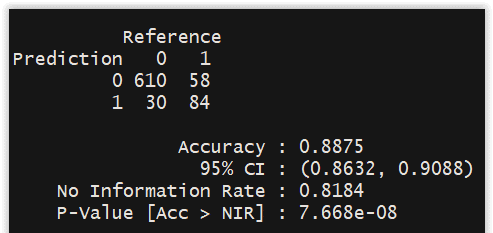
The results remain relatively correct with an accuracy of 89%.
We will decrypt this matrix.
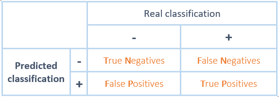
In our DATA SEO LABS training, we have noticed that it is easy to understand the true positives and true negatives, but it is complicated to understand the false negatives and false positives.
Looking back, it’s a concept issue. When you read false negatives, you have to read: Negative prediction but false
If you read false positives, then you should read: Positive prediction but false
This makes it easy to place the different numbers correctly and calculate the accuracy rate.
Accuracy = (TN + TP) / ( TN + FN + FP + TP) = 694 / 782 = 0.88746
Bonus question: how many URLs do you need to get a correct result?
After a few tests, I got good results with at least 500 URLs. You have to make sure that the pages are crawled regularly by the Googlebot.
Step 6: Let’s automate a little bit
Here is the line to repeat steps 2,3,4 and 5 in one line of code:
datasetMatAll <- left_join(pages_fetched,logs,by="url")
list <- oncrawlTrainModel(datasetMatAll)
In the settings, you can also pass the number of iterations that the algorithm must perform.
By default, it is 400. The function returns the confusion matrix and ROC curve to measure the reliability of the results.
Now we get to step 7, where we will be able to understand and use the results.
Step 7: DALEX: Descriptive mAchine Learning EXplanations
I’m a fan of DALEX: Descriptive mAchine Learning EXplanations to understand ML models. The name is inspired by a recurring villain of Doctor Who who spends his time saying: Explain! https://www.youtube.com/watch?v=JYqjcHYTQgQ

Models are becoming more and more sophisticated due to the increasing computing power of computers and the complexity of data sources.
When you take XgBoost or neural networks, for example, they are configured with thousands or even millions of possibilities.
It is difficult to understand the relationship between the input variables and the model results, it is called a black box. These ML models are used because of their high performance, but their lack of interpretability remains one of their biggest weaknesses.
Unfortunately for SEO, we need to know the impact of each variable on the final model predictions.
This is where the DALEX package comes in: https://pbiecek.github.io/DALEX_docs/
This package allows us to develop an understanding of a very large number of ML models.
Using DALEX
Machine Learning’s “black box” models can have very different structures. The DALEX function creates a unified representation of a model, which will be used to explain the different factors of importance.
library("DALEX")
explainer_xgb <- explain(model,
                          data = data.matrix(X_wt),
                          y = data.matrix(y),
                          label = "xgboost")
 explainer_xgb
That’s it! Your model is ready to be explained.
Let’s now look at the factors of importance for this dataset
The “variable_importance” function allows you to list the variables that have a significant influence on the result.
vd_xgb <- variable_importance(explainer_xgb, type = "raw")
plot(vd_xgb)
explainer_xgb: The model to be explained by the explain function
loss_function: A function that will be used to evaluate important variables.
type: The type of transformation that should be applied for dropout loss.
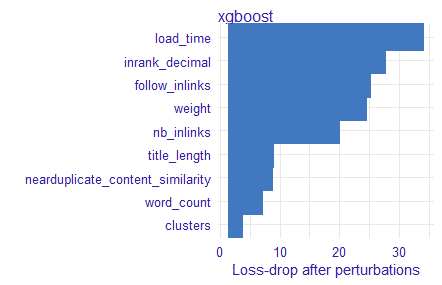
Here is what we get with OnCrawl data. In fact, the DALEX package will create significant perturbations on the input variables and observe the output results by ranking them in order of impact.
Let’s explain the most important variables
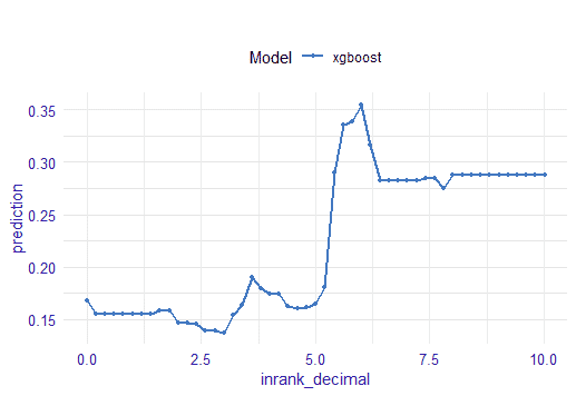
Then there is the “single_variable” function that calculates the average response of the model based on a single selected variable. Now the DALEX package will vary this input parameter to see if the prediction of whether the page is “superactive” increases or decreases.
sv_xgb_satisfaction_level  <- single_variable(explainer_xgb,
                                               variable = "inrank_decimal ", type = "pdp")
plot(sv_xgb_satisfaction_level)
explainer_xgb: The model to be explained
type: The type of marginal response to be calculated.
Currently, for numerical variables, the DALEX package uses the “PDP” package (Partial Dependency and Accumulated Local Effects) ( Url to be added)
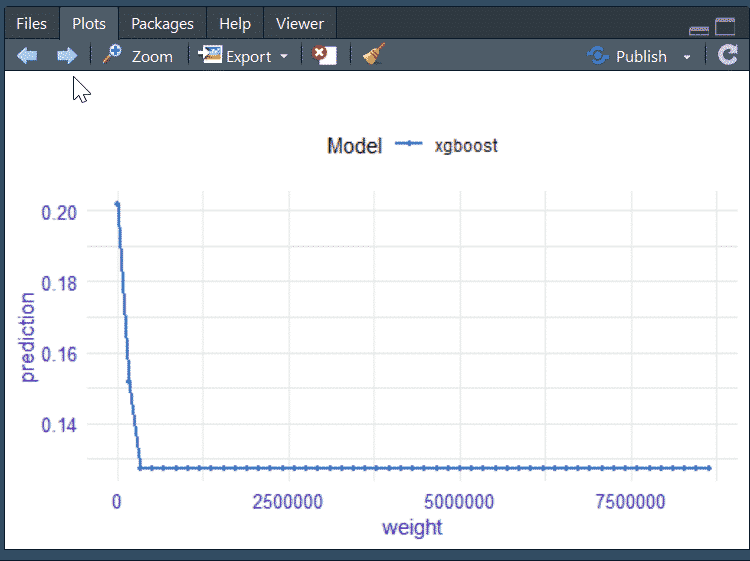
For the Inrank (or internal page rank), we have the following graph but you can also use the table with all the notable values.
For example, here we understand that pages that have an Inrank less than 6 go from a prediction accuracy of 0.3 to 0.15, which is indicative of the importance of the website’s internal linking.
For users of the R oncrawlR package
Everything can be done in 2 lines of code!
list <- oncrawlTrainModel(datasetMatAll,500)
oncrawlExplainModel(list$model, list$x, list$y, 8)
Then, you can view and export thresholds and images using the RStudio View tab. You have buttons to scroll through the graphs and a button to export the graphs to your SEO audits or slides. The parameter “8” in the oncrawlExplainModel function simply allows you to specify how many important variables you want to explain.
Mission accomplished
Now you have determined the main variables of importance for your site and you have established the thresholds necessary to influence your SEO traffic. Be careful: each site will have different variables of importance and different thresholds. This is absolutely not a one-size-fits-all approach, but rather a scientific one. If the accuracy is high, you can guarantee the results.
The next step will be dedicated to automatically creating an SEO audit in a well-presented PowerPoint format that respects your brand’s fonts and logo. This report will use OnCrawl graphs over the period of your choice and integrate the important variables and thresholds that should be addressed first. You will be able to add your comments and devote more time to monitoring, analysis and strategy rather than to collecting and preparing the data.