
We have got a lot of data from previous articles. Now it is time to format them and distribute them in a PowerPoint file by respecting your fonts, your content, your logo, and your colors.

If you already have a neat PowerPoint template, it is easy to industrialize the process and focus your energy on the analyses. Ready to save time?
PowerPoint Generation
We will use the package R: officeR which runs on Mac and PC.
The officeR package allows R users to manipulate Word (.docx) and PowerPoint (*.pptx) documents. It is easy to add images, tables and text to documents. An initial document can be provided; the content, styles and properties of the original document will then be retained. Examples are provided at the end of the article once the data is formatted.
Before starting to use this package, you need to get the data. Here we will see examples based on articles 1, 2 and 3.
Let’s get all the crawls from OnCrawl
If you regularly crawl your site with OnCrawl, it is interesting to study long periods of time. Below we will see an example code to retrieve several crawls.
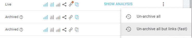
There is no time limit. On the other hand, old crawls can be archived. Sometimes if you go back to old periods, you will have to unarchive them via the OnCrawl platform.
You have the option “un-archive all” for each archived crawl.
Here is an R code that allows you to pick up the last ten crawls of a project. It includes all the functions we saw in article 1 on the OnCrawl API.
listProjectsId <- listProjects()

last_crawl_ids <- unlist(listProjectsId$projects$crawl_ids[2])

last_crawl_top10 <- head(last_crawl_ids, 10)

for (crawlId in last_crawl_top10) {

    crawlInfo <- getCrawl(crawlId)

    date_in_ms <- crawlInfo$crawl$created_at

    sec <- date_in_ms / 1000

    date_format <- as.POSIXct(sec, origin="1970-01-01", tz=Sys.timezone())

    date_format <- substr(date_format,1,10)

    pages <- listPages(crawlId)

    assign(paste("crawl_d_", date_format, sep = ""), pages)

}
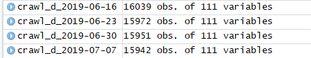
Each crawl is stored in memory under the variable name crawl_d_DATE to allow us to calculate the metrics we are interested in.
Below, an example:
Let’s start extracting the first metrics
With R or Python, it is easy to calculate your metrics when the data has been correctly collected and qualified.
With R, I recommend the Dplyr package.
With Python, I recommend the Pandas library.
Here is a non-exhaustive list of metrics.
We will see concrete examples later in the article.
| Metric | R with Dplyr |
| duplicateDescription | nrow(filter(result, description_evaluation == « duplicated »)) |
| duplicateTitle | nrow(filter(result, title_evaluation == « duplicated »)) |
| nearDuplicatePages | nrow(filter(result, nearduplicate_content == TRUE)) |
| poorContent | nrow(filter(result, word_count_range == « xs »)) |
| incompleteOpenGraph | nrow(filter(result, ogp_evaluation != « complete »)) |
| notCanonical | nrow(filter(result, canonical_evaluation != « matching »)) |
| indexable | nrow(filter(result, fetched == TRUE && meta_robots_index == TRUE)) – nrow(filter(result, canonical_evaluation == « not_matching »)) – nrow(filter(result, status_code != « 200 »)) |
| code3xx | nrow(filter(result, status_code == « 301 »)) |
| code4xx | nrow(filter(result, status_code == « 404 »)) |
| code5xx | nrow(filter(result, status_code == « 500 »)) |
| pages_in_structure | nrow(filter(result, depth>0)) |
| indexable_canonical_pages | nrow(filter(result, meta_robots_index == « True » & status_code_range == « ok » & canonical_evaluation != « not_matching » & fetched == « True »)) |
| seo_active_orphan_pages | nrow(filter(result, is.na(depth) & analytics_entrances_seo_google >0 )) |
| seo_active_traffic | nrow(filter(result, analytics_entrances_seo_google >0 )) |
| seo_visits_google | sum(result$analytics_entrances_seo_google) |
Each time, I store the metric in a data.frame with its date, value and unique name.
For example:
res <- rbind(res, data.frame(date=date,

     value=seo_visits_orphan_pages_google,

     metric="Visits orphan pages Google"))
The classic: Growth rate
I had the chance to work for two big companies (a online media site and an e-commerce site) and there is a very strong common point that interested both steering committees: the growth rates.
In each case, data analysts must juggle with easy-to-read calculations of growth rates, colours and indicators.

That’s great, but we lose track of the trend because we often focus on easy-to-explain time data, such as year or month.
That’s why it’s important to add sparklines to track trends.
A “sparkline” is a small graph in a column that provides a visual representation of the data. It is widely used to show trends in a series of values, such as seasonal increases or decreases, business cycles, or to highlight maximum and minimum values.
Introduction to the formatable package
There is a package that allows breathtaking presentations from any table in R format. With this package, it is easy to add sparklines and indicators.
If you want to know more, I invite you to read this article: https://www.littlemissdata.com/blog/prettytables
In the oncrawlR package, there is now a function that will do the work for you from the data we previously created. You can track variations over any period with trends and associated sparklines.
Here is the result:
However, this table is in HTML so the trick is to also use a package that transforms the HTML page into an image so that you can integrate it into your SEO audit.
Everything can be done in one line of code regardless of the number of crawls. The function will draw the sparkline with all the crawls and then display the first and last values, calculate the growth rate, and add the corresponding indicators with the right color.
The function needs 4 arguments: first the name of the dataframe with the three columns mentioned above (date, metric name and metric value), then the name of the image to be created, the size of the image, and the location of the file.
oncrawlCreateDashboard(res, "metricSEO.png", 500, ".")
What to put in an SEO report?
An audit must be concise and effective by focusing on explained and prioritized actions.
You will find a model in the conclusion of this article, but you can, of course, im-prove it. The most important thing is to track metrics by categories, and that is why I mentioned in the second article how to do cross-segment categorization.
In the PowerPoint, you have the details within each category:
- For visits
- For number of pages.
all <- ls()

objects <- all[which(grepl("^crawl_d_", all))]

resGroupByCategory <- data.frame( date=character() , value=integer(), metric=character() )

for (obj in objects) {

   result <- get(obj)

   date <- substr(obj,9,nchar(obj))

   result$metric <- "no match"

   for (j in 1:length(urls)) {

       result$metric[which(stri_detect_fixed(result$urlpath,urls[j],      case_insensitive=TRUE))] <- urls[j]

   }

   resLastCrawlCategory <- group_by(result, metric) %>%

      summarise(value=n()) %>%

       mutate(date=date) %>%

       ungroup()

   resGroupByCategory <- rbind(resGroupByCategory, resLastCrawlCategory )

}

oncrawlCreateDashboard(resGroupByCategory, "metricCategory.png", 500, ".")
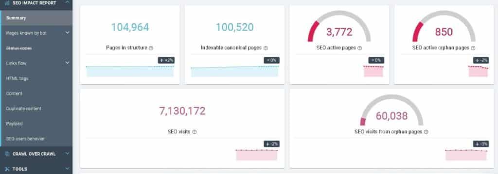
Then there is an SEO Impact Report in OnCrawl that gives you the metrics that have the most impact on your SEO strategies.
Here is an example. Warning: all the numbers below are merely examples.
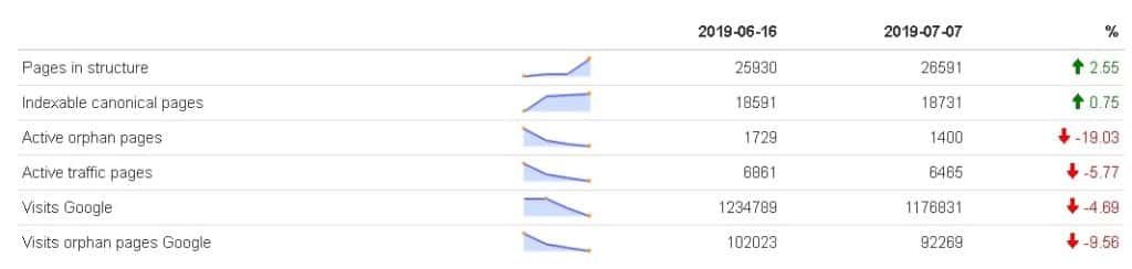
So here is the code that allows you to retrieve your metrics by focusing only on traffic from Google. Later, we will be able to insert it into a PowerPoint.
We find the R code with Dplyr which allows us to calculate each metric.
all <- ls()

objects <- all[which(grepl("^crawl_d_", all))]

res <- data.frame(date=character(), value=integer(), metric=character() )

for (obj in objects)  {
result <- get(obj)
date <- substr(obj,9,nchar(obj))
pages_in_structure <- nrow(filter(result,depth>0))

res <- rbind(res, data.frame(date=date, value=pages_in_structure,

metric="Pages in structure"))

indexable_canonical_pages <-nrow(filter(result, meta_robots_index == "True" &

status_code_range == "ok" & canonical_evaluation !="not_matching" & fetched == "True"))

res <- rbind(res, data.frame(date=date, value=indexable_canonical_pages, metric="Indexable canonical pages"))

#traffic mais depth=0 = orphan
seo_active_orphan_pages <- nrow(filter(result, is.na(depth) & analytics_entrances_seo_google >0 ))

res <- rbind(res, data.frame(date=date, value=seo_active_orphan_pages, metric="Active orphan pages"))

seo_active_traffic <- nrow(filter(result, analytics_entrances_seo_google

res <- rbind(res, data.frame(date=date, value=seo_active_traffic, metric="Active traffic pages"))

seo_visits_google <- sum(result$analytics_entrances_seo_google)

res <- rbind(res, data.frame(date=date, value=seo_visits_google,metric="Visits Google"))

seo_visits_orphan_pages_google <- sum(filter(result, is.na(depth) & analytics_entrances_seo_google>0 )$analytics_entrances_seo_google)

res <- rbind(res, data.frame(date=date, value=seo_visits_orphan_pages_google, metric="Visits orphan pages Google"))

}

oncrawlCreateDashboard(res, "metricSEO.png", 500, ".")
Here is the final result:

Adding ranking factors and thresholds
Now we can insert the ranking factors and explain the main thresholds we have generated in Article 3.
list <- oncrawlTrainModel(datasetMatAll,200)

ggsave("variable_importance.jpg",model$plot)

#please be patient !
model <- oncrawlExplainModel(list$model, list$x, list$y, 3, ".")

list_importance_variable <- model$factors

# explain variable 1
factor_top <-list_importance_variable[1]oncrawlCreateGraph(factor_top,"factor_top1.jpg",2, 1,".")

#explain variable 2
factor_top <- list_importance_variable[2]oncrawlCreateGraph(factor_top,"factor_top2.jpg",2, 1,".")

#explain variable 3
factor_top <- list_importance_variable[3]

oncrawlCreateGraph(factor_top,"factor_top3.jpg",
 2, 1,".")
In this example, I limited it to 3 variables because the more ranking factors you handle, the more time you spend, and the more the budget will be important. I’ll let you set the right limit.
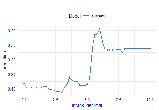
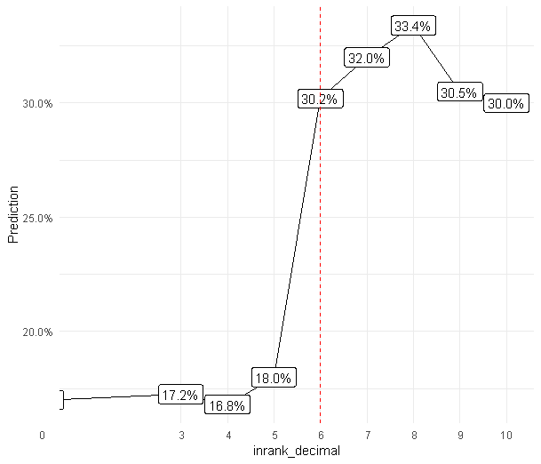
However, I have rebuilt the graphs explaining the important variables with DALEX because they were not explicit enough. Now, a function detects sudden threshold changes and indicates the values you should track.
Here is the result:
BEFORE
AFTER
Let’s generate the PowerPoint
In this section we will look at the code to generate a PowerPoint in R. If you want to do more sophisticated operations on your slides, such as adding new slides, the documentation is here: https://cran.r-project.org/web/packages/officer/vignettes/powerpoint.html
Reading a PowerPoint
doc <- read_pptx(“CHEMIN”)
Important tip
You have to move around in the slides and retrieve the common elements in order to know where to place your texts or images
Recover all elements on slide 1
sumdoc <- slide_summary(doc, index = 1)
Indicate that we’re modifying slide 1: very important the next steps
doc$cursor <- 1
Adding text
Here is an example with a date.
doc <- ph_add_text(x=doc
              ,str=format(Sys.Date())
              ,ph_label = "Google Shape;59;p13"
              ,pos="before"
              ,style = fp_text(color="white",
                               font.size=36,
                               font.family="Proxima Nova",
                               bold=TRUE
                               )
              )
This ph_add_text function allows you to place text with the current date in the element: “Google Shape;59;p13” which is defined in the “slide_summary” function above. The “style” arguments set the style of the text; you can adapt them to your template.
Adding a picture in your slide
Here is an example in which I add an image to slide number 4.
It is up to you to place the image using the variables left and top and to define the size in height and width.
sumdoc <- slide_summary(doc, index = 4)

 doc$cursor <- 4

 add img

 img.file <- file.path( "metricSEO.png" )

 if( file.exists(img.file) ){

   doc <- ph_with_img_at(x = doc, src = img.file,

                           height = 2, width = 5,

                           left = 4.9, top = 1

                         )

 }
Saving the result
The print function allows you to save the file in the directory of your choice.
If nothing is specified, the PowerPoint will be saved in the current project directory.
print(doc, target = “SEO Report2.pptx” )
Mission accomplished
Do you want to download the final result? It’s available in exchange for a tweet because it took a long time to create. Using the following link, you will get the code to generate it and an example of the generated PowerPoint.
These four Data-SEO articles have demonstrated how to automate the following key steps with machine learning:
- preparing and cleaning up data
- classifying your documents
- finding key information in the “black box” models
- creating dashboards based on the identified variables
Because of the millions of combinations of variables, it would take too long for a human to do these steps manually.
In fact, computer-aided analysis is already implemented in many BI tools, which are able to provide you with suggestions on the right visual according to the selected measurements and dimensions.
By 2025, I believe we will move from passive tools where humans seek information to active tools where information seeks its consumer through highly sophisticated algorithms.
The future will mainly be played out in active algorithms that are constantly looking for trends, outliers and opportunities and that will trigger the best actions for your sites. OnCrawl remains a pioneer in this field through the richness of the platform.
What’s your take on this vision of the future? Feel free to leave me a comment on this series of articles.
Thank you for following my articles on OnCrawl data. I am currently working on preparing the Python equivalents to these R functions, as well as creating the accompanying training that will be dedicated to OnCrawl data and all use cases.
I wanted to end with a thank you.
Thanks to Rebecca (@Rbbrbl) for her brilliant advice and review of each article.
Thanks to Alice (@aaliceroussel) for her feedback.
Thanks to François, Tanguy and Philippe for making the SEO Technique so accessible.